Mean-Field Dynamics
In this tutorial we discuss to use TEMPO and the process tensor approach to compute the dynamics of a many-body system of the type introduced in [FowlerWright2022] (PhysRevLett.129.173001 (2022) / arXiv:2112.09003).
launch binder (runs in browser),
read through the text below and code along.
Contents:
Background and introduction
many-body system and environment Hamiltonians
system Hamiltonian and field equation of motion after the mean-field reduction
Creating time-dependent system with field and bath objects
TEMPO computation for single dynamics
PT-TEMPO computation for multiple sets of dynamics
We firstly import OQuPy and other useful packages:
import sys
sys.path.insert(0,'..')
import oqupy
import numpy as np
import matplotlib.pyplot as plt
Check the current OQuPy version; mean-field functionality was introduced in version 0.3.0 and revised in its current format in 0.4.0.
oqupy.__version__
'0.5.0'
The following matrices will be useful below:
sigma_z = oqupy.operators.sigma("z")
sigma_plus = oqupy.operators.sigma("+")
sigma_minus = oqupy.operators.sigma("-")
1. Background and introduction
Our goal will be to reproduce a line from Fig. 2a. of [FowlerWright2022] which shows the photon number dynamics for the driven-dissipative system of molecules in a single-mode cavity.
Many-body system and environment Hamiltonian
The Hamiltonian describing the many-body system with one-to-all light-matter coupling is
Together with the vibrational environment of each molecule,
This is taken to be a continuum of low frequency modes with coupling characterized by a spectral density with a ‘Gaussian’ cut-off
where \(\alpha=0.25\) is the unit-less coupling strenght and \(\hbar \nu_c = 0.15\) eV is a cutoff frequency for the environment of the BODIPY-Br molecule considered in the Letter. For the numericla simulation we here choose to express all frequencies as angular frequencies in the units of \(\frac{1}{\text{ps}}\) (setting \(\hbar = k_B = 1\)) and all times in units of ps. The parameters relevant to Fig. 2a. given in those units are:
\(\nu_c = 0.15 \text{eV} = 227.9 \frac{1}{\text{ps}}\) … environment cutoff frequency
\(T = 300 \text{K} = 39.3 \frac{1}{\text{ps}}\) … environment temperature
\(\omega_0 = 0.0 \frac{1}{\text{ps}}\) … two-level system frequency *
\(\omega_c = -0.02 \text{eV} = -30.4 \frac{1}{\text{ps}}\) … bare cavity frequency
\(\Omega = 0.2 \text{eV} = 303.9 \frac{1}{\text{ps}}\) … collective light-matter coupling
together with the rates
\(\kappa = 15.2 \frac{1}{\text{ps}}\) … field decay
\(\Gamma_\downarrow = 15.2 \frac{1}{\text{ps}}\) … electronic dissipation
\(\Gamma_\uparrow \in (0.2\Gamma_\downarrow, 0.8\Gamma_\downarrow)\) … electronic pumping
The latter appear as prefactors for Markovian terms in the quantum master equation for the total density operator
As indicated, it is the pump strength \(\Gamma_\uparrow\) that is varied to generate the different lines of Fig. 2a. In this tutorial we generate the \(\Gamma_\uparrow=0.8\,\Gamma_\downarrow\) line using the TEMPO method, and then the Process Tensor approach to calculate all of the lines efficiently.
The following code box defines each of the above parameters.
* N.B. for calculating the dynamics only the detuning \(\omega_c-\omega_0\) is relevant, so we set \(\omega_0=0\) for convenience.
alpha = 0.25
nu_c = 227.9
T = 39.3
omega_0 = 0.0
omega_c = -30.4
Omega = 303.9

kappa = 15.2
Gamma_down = 15.2
Gamma_up = 0.8 * Gamma_down
System Hamiltonian and field equation of motion after the mean-field reduction
The mean-field approach is based on a product-state ansatz for the total density operator \(\rho\),
where \(\text{Tr}_{\otimes{i}}\) denotes a partial trace taken over the Hilbert space of all two-level systems and \(\text{Tr}_{a, \otimes{j\neq i}}\) the trace over the photonic degree of freedom and all but the \(i^{\text{th}}\) two-level system. As detailed in the Supplement of the Letter, after rescaling the field \(\langle a \rangle \to \langle a \rangle/\sqrt{N}\) (\(\langle a \rangle\) scales with \(\sqrt{N}\) in the lasing phase), the dynamics are controlled by the mean-field Hamiltonian \(H_{\text{MF}}\) for a single molecule,
together with the equation of motion for the field \(\langle a \rangle\),
Therefore in order to calculate the dynamics we need to encode the
field’s equation of motion in addition to the Hamiltonian for a single
two level-system \(\rho_i\). This is done in OQuPy using the
MeanFieldSystem class.
2. Creating time-dependent system with field and bath objects
A MeanFieldSystem object is initialised with a field equation of
motion and one or more TimeDependentSystemWithField which objects in
turn are characterised by Hamiltonians with both time and field
depedence. In the present example, we need only one
TimeDependentSystemWithField, for the single molecule Hamiltonian
\(H_{\text{MF}}\), but other problems may require multiple such
objects e.g. to encode different types of molecules.
field_eom(t, state_list, a) which takes as arguments
time, a list of states as square matrices (numpy ndarrays) and a
field - a function H_MF(t, a) which takes a time and a fieldSince positional arguments are used in the definition of these
functions, the order of arguments matter, whereas their names do not. In
particular, both functions must have a time variable for their first
argument, even if there happens to be no explicit time-dependence in the
problem (there is no ‘SystemWithField’ class in OQuPy).
def H_MF(t, a):
    return 0.5 * omega_0 * sigma_z +\
        0.5 * Omega * (a * sigma_plus + np.conj(a) * sigma_minus)
def field_eom(t, state_list, a):
    state = state_list[0]
    expect_val = np.matmul(sigma_minus, state).trace()
    return -(1j * omega_c + kappa) * a - 0.5j * Omega * expect_val
Note that the second argument of field_eom must be a list, even in
the case of a single TimeDependentSystemWithField object (this
requirement is a feature of most functionality involving the
MeanFieldSystem class, as we will see below). Thus, in order to
compute the expectation \(\langle \sigma^- \rangle\) we took the
first element of this list - a \(2\times2\) matrix - before
multiplying by \(\sigma^-\) and taking the trace.
It is a good idea to test these functions:
test_field = 1.0+1.0j
test_time = 0.01
test_state_list = [ np.array([[0.0,2j],[-2j,1.0]]) ]
print('H_eval =', H_MF(test_time, test_field))
print('EOM_eval =', field_eom(test_time, test_state_list, test_field))
H_eval = [[  0.    +0.j   151.95+151.95j]
 [151.95-151.95j   0.    +0.j  ]]
EOM_eval = (258.29999999999995+15.2j)
In, we need to specify Lindblad operators for the pumping and dissipation processes:
gammas = [ lambda t: Gamma_down, lambda t: Gamma_up]
lindblad_operators = [ lambda t: sigma_minus, lambda t: sigma_plus]
Here the rates and Lindblad operators must be callables taking a single
argument - time - again, even though in our example there is no explicit
time-dependence. The TimeDependentSystemWithField object is then
constructed as
system = oqupy.TimeDependentSystemWithField(
        hamiltonian=H_MF,
        gammas=gammas,
        lindblad_operators=lindblad_operators)
and the encompasing MeanFieldSystem as
system_list = [system] # a list of TimeDependentiSystemWithField objects
mean_field_system = oqupy.MeanFieldSystem(
                    system_list=system_list,
                    field_eom=field_eom)
where we note the single system must be placed in a list,
system_list, before being passed to the MeanFieldSystem
constructor.
Correlations and a Bath object are created in the same way as in any other TEMPO computation (refer to preceding tutorials), although here we will need the Bath in a list:
correlations = oqupy.PowerLawSD(alpha=alpha,
                                zeta=1,
                                cutoff=nu_c,
                                cutoff_type='gaussian',
                                temperature=T)
bath = oqupy.Bath(0.5 * sigma_z, correlations)
bath_list = [bath]
3. TEMPO computation for single dynamics
For our simulations we use the same initial conditions for the system and state used in the Letter:
initial_field = np.sqrt(0.05) # Note n_0 = <a^dagger a>(0) = 0.05
initial_state = np.array([[0,0],[0,1]]) # spin down
initial_state_list = [initial_state] # initial state must be provided in a list
To reduce the computation time we simulate only the first 0.3 ps of the dynamics with much rougher convergence parameters compared to the letter.
tempo_parameters = oqupy.TempoParameters(dt=3.2e-3, tcut=64e-3, epsrel=10**(-5))
start_time = 0.0
end_time = 0.3
The oqupy.MeanFieldTempo.compute method may then be used to compute
the dynamics in an analogous way a call to oqupy.Tempo.compute is
used to compute the dynamics for an ordinary System:
tempo_sys = oqupy.MeanFieldTempo(mean_field_system=mean_field_system,
                                 bath_list=[bath],
                                 initial_state_list=initial_state_list,
                                 initial_field=initial_field,
                                 start_time=start_time,
                                 parameters=tempo_parameters,
                                 unique=True)
mean_field_dynamics = tempo_sys.compute(end_time=end_time)
--> TEMPO-with-field computation:
100.0%   93 of   93 [########################################] 00:00:06
Elapsed time: 6.3s
MeanFieldTempo.compute returns a MeanFieldDynamics object
containing an array of timesteps, the field values at these timesteps,
and a list of ordinary Dynamics objects, one for each of
TimeDependentSystemWithField objects (here only one):
times = mean_field_dynamics.times
fields = mean_field_dynamics.fields
system_dynamics = mean_field_dynamics.system_dynamics[0]
states = system_dynamics.states
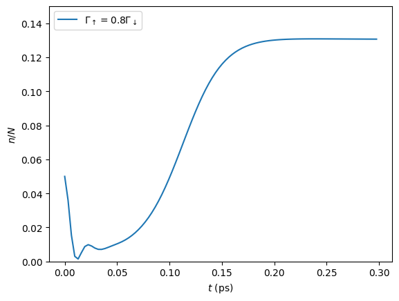
We plot a the square value of the fields i.e. the photon number, producing the first part of a single line of Fig. 2a.:
n = np.abs(fields)**2
plt.plot(times, n, label=r'$\Gamma_\uparrow = 0.8\Gamma_\downarrow$')
plt.xlabel(r'$t$ (ps)')
plt.ylabel(r'$n/N$')
plt.ylim((0.0,0.15))
plt.legend(loc='upper left')
<matplotlib.legend.Legend at 0x7fdb289b2b90>
If you have the time you can calculate the dynamics to
\(t=1.3\,\text{ps}\) as in the Letter and check that, even for these
very rough parameters, the results are reasonably close to being
converged with respect to dt, tcut and epsrel.
While you could repeat the TEMPO computation for each pump strength \(\Gamma_\uparrow\) appearing in Fig. 2a., a more efficient solution for calculating dynamics for multiple sets of system parameters (in this case Lindblad rates) is provided by PT-TEMPO.
4. PT-TEMPO computation for multiple sets of dynamics
The above calculation can be performed quickly for many-different pump strengths \(\Gamma_\uparrow\) using a single process tensor.
As discussed in the Supplement Material for the Letter, there is no guarantee that computational parameters that gave a set of converged results for the TEMPO method will give converged results for a PT-TEMPO calculation. For the sake of this tutorial however let’s assume the above parameters continue to be reasonable. The process tensor to time \(t=0.3\,\text{ps}\) is calculated using these parameters and the bath via
process_tensor = oqupy.pt_tempo_compute(bath=bath,
                                        start_time=0.0,
                                        end_time=0.3,
                                        parameters=tempo_parameters)
--> PT-TEMPO computation:
100.0%   93 of   93 [########################################] 00:00:01
Elapsed time: 1.1s
Refer the Time Dependence and PT-TEMPO tutorial for further discussion of the process tensor.
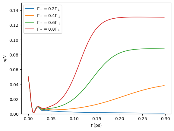
To calculate the dynamics for the 4 different pump strengths in Fig.
2a., we define a separate MeanFieldSystem object for each pump
strength. Only the gammas array needs to be modified between sets of
constructor calls:
pump_ratios = [0.2, 0.4, 0.6, 0.8]
mean_field_systems = []
for ratio in pump_ratios:
    Gamma_up = ratio * Gamma_down
    # N.B. a default argument is used to avoid the late-binding closure issue
    # discussed here: https://docs.python-guide.org/writing/gotchas/#late-binding-closures
    gammas = [ lambda t: Gamma_down, lambda t, Gamma_up=Gamma_up: Gamma_up]
     # Use the same Hamiltonian, equation of motion and Lindblad operators
    system = oqupy.TimeDependentSystemWithField(H_MF,
        gammas=gammas,
        lindblad_operators=lindblad_operators)
    mean_field_system = oqupy.MeanFieldSystem(system_list=[system],
                                             field_eom=field_eom)
    mean_field_systems.append(mean_field_system)
We can then use compute_dynamics_with_field to compute the dynamics
at each \(\Gamma_\uparrow\) for the particular initial condition
using the process tensor (now in a list) calculated above:
t_list = []
n_list = []
for i, mean_field_system in enumerate(mean_field_systems):
    mean_field_dynamics = oqupy.compute_dynamics_with_field(
        process_tensor_list=[process_tensor],
        mean_field_system=mean_field_system,
        initial_state_list=[initial_state],
        initial_field=initial_field,
        start_time=0.0)
    t = mean_field_dynamics.times
    fields = mean_field_dynamics.fields
    n = np.abs(fields)**2
    t_list.append(t)
    n_list.append(n)
--> Compute dynamics with field:
100.0%   93 of   93 [########################################] 00:00:04
Elapsed time: 4.2s
--> Compute dynamics with field:
100.0%   93 of   93 [########################################] 00:00:03
Elapsed time: 3.9s
--> Compute dynamics with field:
100.0%   93 of   93 [########################################] 00:00:04
Elapsed time: 4.1s
--> Compute dynamics with field:
100.0%   93 of   93 [########################################] 00:00:04
Elapsed time: 4.0s
Finally, plotting the results:
for i,n in enumerate(n_list):
    ratio = pump_ratios[i]
    label = r'$\Gamma_\uparrow = {}\Gamma_\downarrow$'.format(pump_ratios[i])
    plt.plot(t_list[i], n_list[i], label=label)
plt.xlabel(r'$t$ (ps)')
plt.ylabel(r'$n/N$')
plt.ylim((0.0,0.15))
plt.legend(loc='upper left')
<matplotlib.legend.Legend at 0x7fdb28590d00>
5. Summary
To summarise the classes and methods for calculating mean-field dynamics:
A Hamiltonian with time \(t\) and field \(a\) dependence is used to construct a
TimeDependentSystemWithFieldobjectOne or more
TimeDependentSystemWithFieldobjects and a field equation of motion forms aMeanFieldSystemoqupy.MeanFieldTempo.computeor.compute_dynamics_with_field(process tensor) may be used to calculateMeanFieldDynamicsMeanFieldDynamicscomprises one of more systemDynamicsand a set of field valuesfields.