Time dependence and PT-TEMPO
A quick introduction on how to use the OQuPy package to compute the dynamics of a time dependent quantum system and how to employ the process tensor TEMPO method. We illustrate this by applying TEMPO and PT-TEMPO to a quantum dot driven by a time dependent laser pulse.
launch binder (runs in browser),
read through the text below and code along.
Contents:
Example - Quantum dot driven by a laser pulse
Hamiltonian for driven quantum dot with bosonic environment
Laser pulse / time dependent system
Create time dependent system object
TEMPO computation
Using PT-TEMPO to explore many different laser pulses
First, let’s import OQuPy and some other packages we are going to use
import sys
sys.path.insert(0,'..')

import oqupy
import numpy as np
import matplotlib.pyplot as plt
and check what version of tempo we are using.
oqupy.__version__
'0.5.0'
Let’s also import some shorthands for the spin Pauli operators and density matrices.
sigma_x = oqupy.operators.sigma("x")
sigma_y = oqupy.operators.sigma("y")
sigma_z = oqupy.operators.sigma("z")
up_density_matrix = oqupy.operators.spin_dm("z+")
down_density_matrix = oqupy.operators.spin_dm("z-")
mixed_density_matrix = oqupy.operators.spin_dm("mixed")
Example - Quantum Dot driven by a laser pulse
As a first example let’s try to reconstruct one of the lines in figure 3c of [Fux2021] (Phys. Rev. Lett. 126, 200401 (2021) / arXiv:2101.03071). In this example we compute the time evolution of a quantum dot which is driven with a \(\pi/2\) laser pulse and is strongly coupled to an ohmic bath (spin-boson model).
1. Hamiltonian for driven quantum dot with bosonic environment
We consider a time dependent system Hamiltonian
which may describe transitions between the ground and exciton state driven by a resonant laser pulse (in the rotating frame). Here, \(\Delta(t)\) is the detuning of the laser with respect to the transition and \(\Omega(t)\) is proportional to the electric field of the laser. We further include a bosonic environment
and an interaction Hamiltonian
where \(\hat{\sigma}_i\) are the Pauli operators, and the \(g_k\) and \(\omega_k\) are such that the spectral density \(J(\omega)\) is
Also, let’s assume the initial density matrix of the quantum dot is the ground state
and the bath is initially at temperature \(T\).
We express all frequencies, temperatures and times in units of 1/ps and ps respectively.
\(\omega_c = 3.04 \frac{1}{\mathrm{ps}}\)
\(\alpha = 0.126\)
\(T = 1 K = 0.1309 \frac{1}{\mathrm{ps}\,\mathrm{k}_B}\)
omega_cutoff = 3.04
alpha = 0.126
temperature = 0.1309
initial_state=down_density_matrix
2. Laser pulse / time dependent system
We choose a gaussian laser pulse shape with an adjustable pulse area and pulse width \(\tau\).
def gaussian_shape(t, area = 1.0, tau = 1.0, t_0 = 0.0):
    return area/(tau*np.sqrt(np.pi)) * np.exp(-(t-t_0)**2/(tau**2))
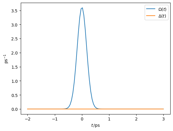
Choosing a pulse area of \(\pi/2\), a pulse width of 245 fs and no detuning, we can check the shape of the laser pulse.
detuning = lambda t: 0.0 * t

t = np.linspace(-2,3,100)
Omega_t = gaussian_shape(t, area = np.pi/2.0, tau = 0.245)
Delta_t = detuning(t)

plt.plot(t, Omega_t,label=r"$\Omega(t)$")
plt.plot(t, Delta_t,label=r"$\Delta(t)$")
plt.xlabel(r"$t\,/\mathrm{ps}$")
plt.ylabel(r"$\mathrm{ps}^{-1}$")
plt.legend()
<matplotlib.legend.Legend at 0x7fc555eaa170>
3. Create time dependent system object
def hamiltonian_t(t):
    return detuning(t)/2.0 * sigma_z \
           + gaussian_shape(t, area = np.pi/2.0, tau = 0.245)/2.0 * sigma_x

system = oqupy.TimeDependentSystem(hamiltonian_t)
correlations = oqupy.PowerLawSD(alpha=alpha,
                                zeta=3,
                                cutoff=omega_cutoff,
                                cutoff_type='gaussian',
                                temperature=temperature)
bath = oqupy.Bath(sigma_z/2.0, correlations)
4. TEMPO computation
With all physical objects defined, we are now ready to compute the dynamics of the quantum dot using TEMPO (using quite rough convergence parameters):
tempo_parameters = oqupy.TempoParameters(dt=0.1, tcut=2.0, epsrel=10**(-4))

tempo_sys = oqupy.Tempo(system=system,
                        bath=bath,
                        initial_state=initial_state,
                        start_time=-2.0,
                        parameters=tempo_parameters)
dynamics = tempo_sys.compute(end_time=3.0)
--> TEMPO computation:
100.0%   50 of   50 [########################################] 00:00:00
Elapsed time: 0.7s
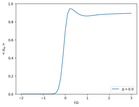
and extract the expectation values \(\langle\sigma_{xy}\rangle = \sqrt{\langle\sigma_x\rangle^2 + \langle\sigma_y\rangle^2}\) for plotting:
t, s_x = dynamics.expectations(sigma_x, real=True)
t, s_y = dynamics.expectations(sigma_y, real=True)
s_xy = np.sqrt(s_x**2 + s_y**2)
plt.plot(t, s_xy, label=r'$\Delta = 0.0$')
plt.xlabel(r'$t\,\Omega$')
plt.ylabel(r'$<\sigma_{xy}>$')
plt.ylim((0.0,1.0))
plt.legend(loc=4)
<matplotlib.legend.Legend at 0x7fc553bb6e30>
5. Using PT-TEMPO to explore many different laser pulses
If we want to do the same computation for a set of different laser pulses (and thus different time dependent system Hamiltonians), we could repeate the above procedure. However, for a large number of different system Hamiltonians this is impractical. In such cases one may instead use the process tensor approach (PT-TEMPO) wherein the bath influence tensors are computed separately from the rest of the network. This produces an object known as the process tensor which may then be used with many different system Hamiltonians at relatively little cost.
tempo_parameters = oqupy.TempoParameters(dt=0.1, tcut=2.0, epsrel=10**(-4))

process_tensor = oqupy.pt_tempo_compute(bath=bath,
                                        start_time=-2.0,
                                        end_time=3.0,
                                        parameters=tempo_parameters)
--> PT-TEMPO computation:
100.0%   50 of   50 [########################################] 00:00:00
Elapsed time: 0.3s
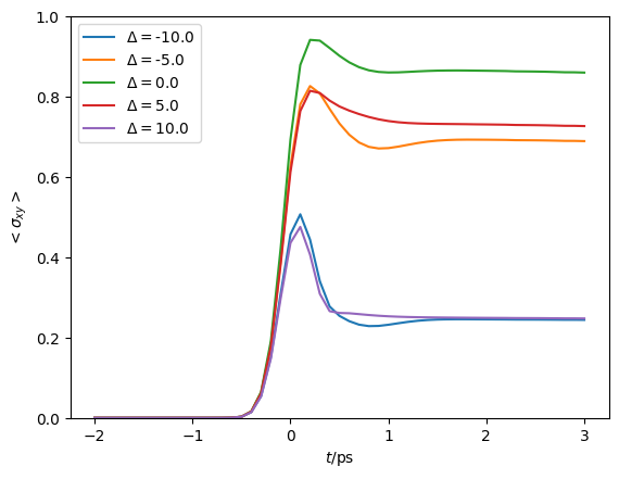
Given we want to calculate \(\langle\sigma_{xy}\rangle(t)\) for 5 different laser pulse detunings, we define a seperate system object for each laser pulse:
deltas = [-10.0, -5.0, 0.0, 5.0, 10.0]
systems = []
for delta in deltas:
    # NOTE: omitting "delta=delta" in the parameter definition below
    #       would lead to all systems having the same detuning.
    #       This is a common python pitfall. Check out
    #       https://docs.python-guide.org/writing/gotchas/#late-binding-closures
    #       for more information on this.
    def hamiltonian_t(t, delta=delta):
        return delta/2.0 * sigma_z \
            + gaussian_shape(t, area = np.pi/2.0, tau = 0.245)/2.0 * sigma_x
    system = oqupy.TimeDependentSystem(hamiltonian_t)
    systems.append(system)
We can then use the process tensor to compute the dynamics for each laser pulse
s_xy_list = []
t_list = []
for system in systems:
    dynamics = oqupy.compute_dynamics(
        process_tensor=process_tensor,
        system=system,
        initial_state=initial_state,
        start_time=-2.0,
        progress_type="silent")
    t, s_x = dynamics.expectations(sigma_x, real=True)
    _, s_y = dynamics.expectations(sigma_y, real=True)
    s_xy = np.sqrt(s_x**2 + s_y**2)
    s_xy_list.append(s_xy)
    t_list.append(t)
    print(".", end="", flush=True)
print(" done.", flush=True)
..... done.
and plot \(\langle\sigma_{xy}\rangle(t)\) for each:
for t, s_xy, delta in zip(t_list, s_xy_list, deltas):
    plt.plot(t, s_xy, label=r"$\Delta = $"+f"{delta:0.1f}")
    plt.xlabel(r'$t/$ps')
    plt.ylabel(r'$<\sigma_{xy}>$')
plt.ylim((0.0,1.0))
plt.legend()
<matplotlib.legend.Legend at 0x7fc553b84bb0>