Quickstart

A quick introduction on how to use the OQuPy package to compute the dynamics of a quantum system that is possibly strongly coupled to a structured environment. We illustrate this by applying the TEMPO method to the strongly coupled spin boson model.

launch binder (runs in browser),
download the jupyter file, or
read through the text below and code along.

Contents:

Example - The spin boson model
- 1. The model and its parameters
- 1. Create system, correlations and bath objects
- 1. TEMPO computation

First, let’s import OQuPy and some other packages we are going to use

import sys
sys.path.insert(0,'..')

import oqupy
import numpy as np
import matplotlib.pyplot as plt

and check what version of tempo we are using.

oqupy.__version__

'0.4.0'

Let’s also import some shorthands for the spin Pauli operators and density matrices.

sigma_x = oqupy.operators.sigma("x")
sigma_y = oqupy.operators.sigma("y")
sigma_z = oqupy.operators.sigma("z")
up_density_matrix = oqupy.operators.spin_dm("z+")
down_density_matrix = oqupy.operators.spin_dm("z-")

Example - The spin boson model

As a first example let’s try to reconstruct one of the lines in figure 2a of [Strathearn2018] (Nat. Comm. 9, 3322 (2018) / arXiv:1711.09641v3). In this example we compute the time evolution of a spin which is strongly coupled to an ohmic bath (spin-boson model). Before we go through this step by step below, let’s have a brief look at the script that will do the job - just to have an idea where we are going:

Omega = 1.0
omega_cutoff = 5.0
alpha = 0.3

system = oqupy.System(0.5 * Omega * sigma_x)
correlations = oqupy.PowerLawSD(alpha=alpha,
                                zeta=1,
                                cutoff=omega_cutoff,
                                cutoff_type='exponential')
bath = oqupy.Bath(0.5 * sigma_z, correlations)
tempo_parameters = oqupy.TempoParameters(dt=0.1, dkmax=30, epsrel=10**(-4))

dynamics = oqupy.tempo_compute(system=system,
                               bath=bath,
                               initial_state=up_density_matrix,
                               start_time=0.0,
                               end_time=15.0,
                               parameters=tempo_parameters)
t, s_z = dynamics.expectations(0.5*sigma_z, real=True)

plt.plot(t, s_z, label=r'$\alpha=0.3$')
plt.xlabel(r'$t\,\Omega$')
plt.ylabel(r'$\langle\sigma_z\rangle$')
plt.legend()

--> TEMPO computation:
100.0%  150 of  150 [########################################] 00:00:08
Elapsed time: 8.5s

<matplotlib.legend.Legend at 0x7fd9c63c8d90>

1. The model and its parameters

We consider a system Hamiltonian

\[H_{S} = \frac{\Omega}{2} \hat{\sigma}_x \mathrm{,}\]

a bath Hamiltonian

\[H_{B} = \sum_k \omega_k \hat{b}^\dagger_k \hat{b}_k \mathrm{,}\]

and an interaction Hamiltonian

\[H_{I} = \frac{1}{2} \hat{\sigma}_z \sum_k \left( g_k \hat{b}^\dagger_k + g^*_k \hat{b}_k \right) \mathrm{,}\]

where \(\hat{\sigma}_i\) are the Pauli operators, and the \(g_k\) and \(\omega_k\) are such that the spectral density \(J(\omega)\) is

\[J(\omega) = \sum_k |g_k|^2 \delta(\omega - \omega_k) = 2 \, \alpha \, \omega \, \exp\left(-\frac{\omega}{\omega_\mathrm{cutoff}}\right) \mathrm{.}\]

Also, let’s assume the initial density matrix of the spin is the up state

\[\begin{split}\rho(0) = \begin{pmatrix} 1 & 0 \\ 0 & 0 \end{pmatrix}\end{split}\]

and the bath is initially at zero temperature.

For the numerical simulation it is advisable to choose a characteristic frequency and express all other physical parameters in terms of this frequency. Here, we choose \(\Omega\) for this and write:

\(\Omega = 1.0 \Omega\)
\(\omega_c = 5.0 \Omega\)
\(\alpha = 0.3\)

Omega = 1.0
omega_cutoff = 5.0
alpha = 0.3

2. Create system, correlations and bath objects

System

\[H_{S} = \frac{\Omega}{2} \hat{\sigma}_x \mathrm{,}\]

system = oqupy.System(0.5 * Omega * sigma_x)

Correlations

\[J(\omega) = 2 \, \alpha \, \omega \, \exp\left(-\frac{\omega}{\omega_\mathrm{cutoff}}\right)\]

Because the spectral density is of the standard power-law form,

\[J(\omega) = 2 \alpha \frac{\omega^\zeta}{\omega_c^{\zeta-1}} X(\omega,\omega_c)\]

with \(\zeta=1\) and \(X\) of the type 'exponential' we define the spectral density with:

correlations = oqupy.PowerLawSD(alpha=alpha,
                                  zeta=1,
                                  cutoff=omega_cutoff,
                                  cutoff_type='exponential')

Bath

The bath couples with the operator \(\frac{1}{2}\hat{\sigma}_z\) to the system.

bath = oqupy.Bath(0.5 * sigma_z, correlations)

3. TEMPO computation

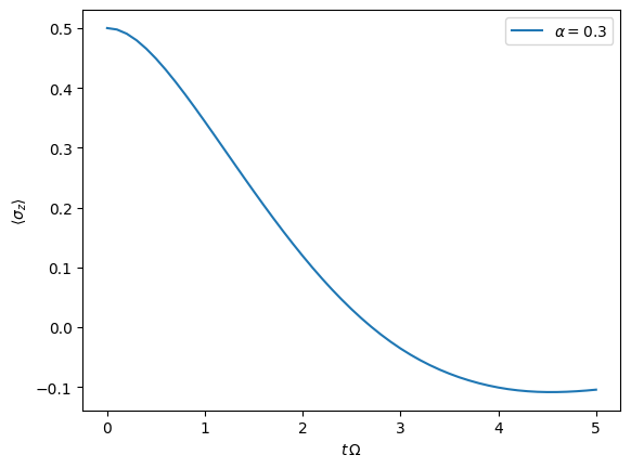
Now, that we have the system and the bath objects ready we can compute the dynamics of the spin starting in the up state, from time \(t=0\) to \(t=5\,\Omega^{-1}\)

dynamics_1 = oqupy.tempo_compute(system=system,
                                   bath=bath,
                                   initial_state=up_density_matrix,
                                   start_time=0.0,
                                   end_time=5.0,
                                   tolerance=0.01)

/home/pip/documents/saints/phd/tempo/OQuPy/tutorials/../oqupy/tempo.py:850: UserWarning: Estimating parameters for TEMPO computation. No guarantee that resulting TEMPO computation converges towards the correct dynamics! Please refer to the TEMPO documentation and check convergence by varying the parameters for TEMPO manually.
  warnings.warn(GUESS_WARNING_MSG, UserWarning)
WARNING: Estimating parameters for TEMPO computation. No guarantee that resulting TEMPO computation converges towards the correct dynamics! Please refer to the TEMPO documentation and check convergence by varying the parameters for TEMPO manually.

--> TEMPO computation:
100.0%   80 of   80 [########################################] 00:00:04
Elapsed time: 4.3s

and plot the result:

t_1, z_1 = dynamics_1.expectations(0.5*sigma_z, real=True)
plt.plot(t_1, z_1, label=r'$\alpha=0.3$')
plt.xlabel(r'$t\,\Omega$')
plt.ylabel(r'$\langle\sigma_z\rangle$')
plt.legend()

<matplotlib.legend.Legend at 0x7fd9c63263e0>

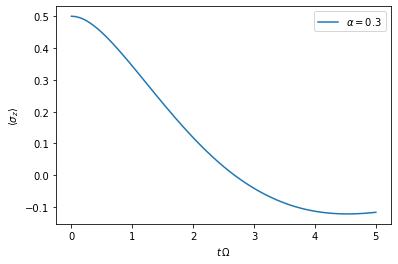
Yay! This looks like the plot in figure 2a [Strathearn2018].

Let’s have a look at the above warning. It said:

WARNING: Estimating parameters for TEMPO calculation. No guarantie that resulting TEMPO calculation converges towards the correct dynamics! Please refere to the TEMPO documentation and check convergence by varying the parameters for TEMPO manually.

We got this message because we didn’t tell the package what parameters to use for the TEMPO computation, but instead only specified a tolerance. The package tries it’s best by implicitly calling the function oqupy.guess_tempo_parameters() to find parameters that are appropriate for the spectral density and system objects given.

TEMPO Parameters

There are three key parameters to a TEMPO computation:

dt - Length of a time step \(\delta t\) - It should be small enough such that a trotterisation between the system Hamiltonian and the environment it valid, and the environment auto-correlation function is reasonably well sampled.
dkmax - Number of time steps \(K \in \mathbb{N}\) - It must be large enough such that \(\delta t \times K\) is larger than the neccessary memory time \(\tau_\mathrm{cut}\).
epsrel - The maximal relative error \(\epsilon_\mathrm{rel}\) in the singular value truncation - It must be small enough such that the numerical compression (using tensor network algorithms) does not truncate relevant correlations.

To choose the right set of initial parameters, we recommend to first use the oqupy.guess_tempo_parameters() function and then check with the helper function oqupy.helpers.plot_correlations_with_parameters() whether it satisfies the above requirements:

parameters = oqupy.guess_tempo_parameters(system=system,
                                          bath=bath,
                                          start_time=0.0,
                                          end_time=5.0,
                                          tolerance=0.01)
print(parameters)

/home/pip/documents/saints/phd/tempo/OQuPy/tutorials/../oqupy/tempo.py:850: UserWarning: Estimating parameters for TEMPO computation. No guarantee that resulting TEMPO computation converges towards the correct dynamics! Please refer to the TEMPO documentation and check convergence by varying the parameters for TEMPO manually.
  warnings.warn(GUESS_WARNING_MSG, UserWarning)
WARNING: Estimating parameters for TEMPO computation. No guarantee that resulting TEMPO computation converges towards the correct dynamics! Please refer to the TEMPO documentation and check convergence by varying the parameters for TEMPO manually.

----------------------------------------------
TempoParameters object: Roughly estimated parameters
 Estimated with 'guess_tempo_parameters()'
  dt                   = 0.0625
  dkmax                = 37
  epsrel               = 2.4846963223857106e-05
  add_correlation_time = None

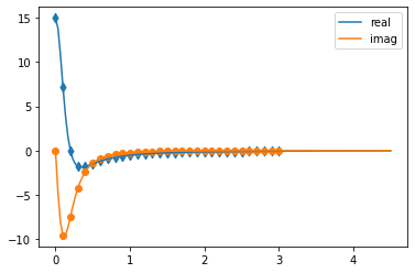
fig, ax = plt.subplots(1,1)
oqupy.helpers.plot_correlations_with_parameters(bath.correlations, parameters, ax=ax)

<AxesSubplot:>

In this plot you see the real and imaginary part of the environments auto-correlation as a function of the delay time \(\tau\) and the sampling of it corresponding the the chosen parameters. The spacing and the number of sampling points is given by dt and dkmax respectively. We can see that the auto-correlation function is close to zero for delay times larger than approx \(2 \Omega^{-1}\) and that the sampling points follow the curve reasonably well. Thus this is a reasonable set of parameters.

We can choose a set of parameters by hand and bundle them into a TempoParameters object,

tempo_parameters = oqupy.TempoParameters(dt=0.1, dkmax=30, epsrel=10**(-4), name="my rough parameters")
print(tempo_parameters)

----------------------------------------------
TempoParameters object: my rough parameters
 __no_description__
  dt                   = 0.1
  dkmax                = 30
  epsrel               = 0.0001
  add_correlation_time = None

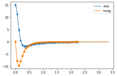
and check again with the helper function:

fig, ax = plt.subplots(1,1)
oqupy.helpers.plot_correlations_with_parameters(bath.correlations, tempo_parameters, ax=ax)

<AxesSubplot:>

We could feed this object into the oqupy.tempo_compute() function to get the dynamics of the system. However, instead of that, we can split up the work that oqupy.tempo_compute() does into several steps, which allows us to resume a computation to get later system dynamics without having to start over. For this we start with creating a Tempo object:

tempo = oqupy.Tempo(system=system,
                      bath=bath,
                      parameters=tempo_parameters,
                      initial_state=up_density_matrix,
                      start_time=0.0)

We can start by computing the dynamics up to time \(5.0\,\Omega^{-1}\),

tempo.compute(end_time=5.0)

--> TEMPO computation:
100.0%   50 of   50 [########################################] 00:00:01
Elapsed time: 1.9s

<oqupy.dynamics.Dynamics at 0x7fd9c53e3760>

then get and plot the dynamics of expecatation values,

dynamics_2 = tempo.get_dynamics()
plt.plot(*dynamics_2.expectations(0.5*sigma_z, real=True), label=r'$\alpha=0.3$')
plt.xlabel(r'$t\,\Omega$')
plt.ylabel(r'$\langle\sigma_z\rangle$')
plt.legend()

<matplotlib.legend.Legend at 0x7fd9c4f45ba0>

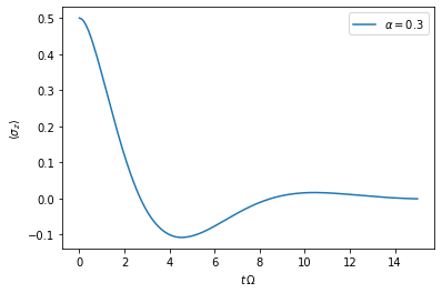
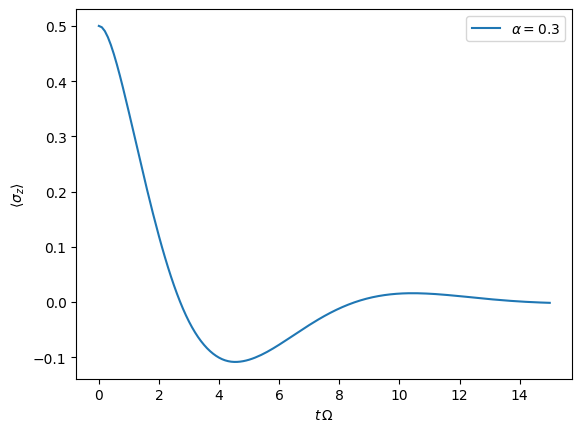
then continue the computation to \(15.0\,\Omega^{-1}\),

tempo.compute(end_time=15.0)

--> TEMPO computation:
100.0%  100 of  100 [########################################] 00:00:06
Elapsed time: 6.1s

<oqupy.dynamics.Dynamics at 0x7fd9c53e3760>

and then again get and plot the dynamics of expecatation values.

dynamics_2 = tempo.get_dynamics()
plt.plot(*dynamics_2.expectations(0.5*sigma_z, real=True), label=r'$\alpha=0.3$')
plt.xlabel(r'$t\,\Omega$')
plt.ylabel(r'$\langle\sigma_z\rangle$')
plt.legend()

<matplotlib.legend.Legend at 0x7fd9c5f05870>

Finally, we note: to validate the accuracy the result it vital to check the convergence of such a simulation by varying all three computational parameters! For this we recommend repeating the same simulation with slightly “better” parameters (smaller dt, larger dkmax, smaller epsrel) and to consider the difference of the result as an estimate of the upper bound of the accuracy of the simulation.